CS224n-2019 Assignment¶

本文档将记录作业中的要点以及问题的答案

课程笔记参见我的博客，并在博客的Repo中提供笔记源文件的下载

Assignment 01¶

逐步完成共现矩阵的搭建，并调用 sklearn.decomposition 中的 TruncatedSVD 完成传统的基于SVD的降维算法
可视化展示，观察并分析其在二维空间下的聚集情况。
载入Word2Vec，将其与SVD得到的单词分布情况进行对比，分析两者词向量的不同之处。
学习使用gensim，使用Cosine Similarity 分析单词的相似度，对比单词和其同义词与反义词的Cosine Distance ，并尝试找到正确的与错误的类比样例
探寻Word2Vec向量中存在的 Independent Bias 问题

Assignment 02¶

1 Written: Understanding word2vec¶

\[ P(O=o | C=c)=\frac{\exp \left(\boldsymbol{u}_{o}^{\top} \boldsymbol{v}_{c}\right)}{\sum_{w \in \mathrm{Vocab}} \exp \left(\boldsymbol{u}_{w}^{\top} \boldsymbol{v}_{c}\right)} \]

\[ J_{\text { naive-softmax }}\left(v_{c}, o, U\right)=-\log P(O=o | C=c) \]

真实(离散)概率分布 $p$ 与另一个分布 $q$ 的交叉熵损失为 $-\sum_i p_{i} \log \left(q_{i}\right)$

Question a

Show that the naive-softmax loss given in Equation (2) is the same as the cross-entropy loss between $y$ and $\hat y$; i.e., show that

\[ -\sum_{w \in Vocab} y_{w} \log \left(\hat{y}_{w}\right)=-\log \left(\hat{y}_{o}\right) \]

Your answer should be one line.

Answer a :

因为 $\textbf{y}$ 是独热向量，所以 $-\sum_{w \in Vocab} y_{w} \log (\hat{y}_{w})=-y_o\log (\hat{y}_{o}) -\sum_{w \in Vocab,w \neq o} y_{w} \log (\hat{y}_{w}) = -\log (\hat{y}_{o})$

Question b

Compute the partial derivative of $J_{\text{naive-softmax}}(v_c, o, \textbf{U})$ with respect to $v_c$. Please write your answer in terms of $\textbf{y}, \hat {\textbf{y}}, \textbf{U}$.

Answer b :

\[ \begin{array}{l} {\frac{\partial J\left(v_{c}, o, U\right)}{\partial v_{c}}} &={-\frac{\partial\left(u_{o}^{T} v_{c}\right)}{\partial v_{c}}+\frac{\partial \left(\log \left(\sum_{w} \exp \left(u_{w}^{T} v_{c}\right)\right)\right)}{\partial v_{c}}} \\ &={-u_{o}+\frac{1}{\sum_{w} \exp \left(u_{w}^{T} v_{c}\right)}} \frac{\partial \left(\sum_{w} \exp \left(u_{w}^{T} v_{c}\right)\right)}{\partial v_{c}} \\ &={-u_{o}+\sum_{w} \frac{\exp \left(u_{w}^{T} v_{c}\right)u_w}{\sum_{w} \exp \left(u_{w}^{T} v_{c}\right)}} \\ &={-u_{o}+\sum_{w} p(O=w | C=c)u_{w}} \\ &={-u_{o}+\sum_{w} \hat{y_w} u_{w}} \\ &={U(\hat{y}-y)} \end{array} \]

Question c

Compute the partial derivatives of $J_{\text{naive-softmax}}(v_c, o, \textbf{U})$ with respect to each of the ‘outside' word vectors, $u_w$'s. There will be two cases: when $w = o$, the true ‘outside' word vector, and $w \neq o$, for all other words. Please write you answer in terms of $\textbf{y}, \hat {\textbf{y}}, \textbf{U}$.

Answer c : $$ \begin{array}{l} {\frac{\partial J\left(v_{c}, o, U\right)}{\partial u_{w}}}
&={-\frac{\partial\left(u_{o}^{T} v_{c}\right)}{\partial u_{w}}+\frac{\partial \left(\log \left(\sum_{w} \exp \left(u_{w}^{T} v_{c}\right)\right)\right)}{\partial u_{w}}} \end{array} $$

When $w \neq o$ :

\[ \begin{array}{l} {\frac{\partial J\left(v_{c}, o, U\right)}{\partial u_{w}}} &= 0 + p(O=w | C=c) v_{c} \\ &=\hat{y}_{w} v_{c} \end{array} \]

When $w = o$ :

\[ \begin{array}{l} {\frac{\partial J\left(v_{c}, o, U\right)}{\partial u_{w}}} &= -v_c + p(O=o | C=c) v_{c} \\ &=\hat{y}_{w} v_{c} - v_c \\ &=(\hat{y}_{w} - 1)v_c \end{array} \]

Then :

\[ {\frac{\partial J\left(v_{c}, o, U\right)}{\partial U}} = v_c(\hat y - y)^T \]

Question d

The sigmoid function is given by the follow Equation :

\[ \sigma(x)=\frac{1}{1+e^{-x}}=\frac{e^{x}}{e^{x}+1} \]

Please compute the derivative of $\sigma (x)$ with respect to $x$, where $x$ is a vector.

Answer d :

\[ \begin{array}{l} \frac{\partial \sigma(x_i)}{\partial x_i} &=\frac{1}{(1+\exp (-x_i))^{2}} \exp (-x_i)=\sigma(x_i)(1-\sigma(x_i)) \\ \frac{\partial \sigma(x)}{\partial x} &= \left[\frac{\partial \sigma\left(x_{j}\right)}{\partial x_{i}}\right]_{d \times d} \\ &=\left[\begin{array}{cccc}{\sigma^{\prime}\left(x_{1}\right)} & {0} & {\cdots} & {0} \\ {0} & {\sigma^{\prime}\left(x_{2}\right)} & {\cdots} & {0} \\ {\vdots} & {\vdots} & {\vdots} & {\vdots} \\ {0} & {0} & {\cdots} & {\sigma^{\prime}\left(x_{d}\right)}\end{array}\right] \\ &=\text{diag}(\sigma^\prime(x)) \end{array} \]

Question e

Now we shall consider the Negative Sampling loss, which is an alternative to the Naive Softmax loss. Assume that $K$ negative samples (words) are drawn from the vocabulary. For simplicity of notation we shall refer to them as $w_{1}, w_{2}, \dots, w_{K}$ and their outside vectors as $u_{1}, \dots, u_{K}$. Note that $o \notin\left\{w_{1}, \dots, w_{K}\right\}$. For a center word $c$ and an outside word $o$, the negative sampling loss function is given by:

\[ J_{\text { neg-sample }}\left(v_{c}, o, U\right)=-\log \left(\sigma\left(u_{o}^{\top} v_{c}\right)\right)-\sum_{k=1}^{K} \log \left(\sigma\left(-u_{k}^{\top} v_{c}\right)\right) \]

for a sample $w_{1}, w_{2}, \dots, w_{K}$, where $\sigma(\cdot)$ is the sigmoid function.

Please repeat parts b and c, computing the partial derivatives of $J_{\text { neg-sample }}$ respect to $v_c$, with respect to $u_o$, and with respect to a negative sample $u_k$. Please write your answers in terms of the vectors $u_o, v_c,$ and $u_k$, where $k \in[1, K]$. After you've done this, describe with one sentence why this loss function is much more efficient to compute than the naive-softmax loss. Note, you should be able to use your solution to part (d) to help compute the necessary gradients here.

Answer e :

For $v_c$ :

\[ \begin{array}{l} \frac{\partial J_{\text {neg-sample}}}{\partial v_c} &=(\sigma(u_o^T v_c) - 1) u_o + \sum_{k=1}^{K}\left(1-\sigma\left(-u_{k}^{T} v_{c}\right)\right) u_{k} \\ &= (\sigma(u_o^T v_c) - 1) u_o+ \sum_{k=1}^{K}\sigma\left(u_{k}^{T} v_{c}\right) u_{k} \end{array} \]

For $u_o$, Remeber : $o \notin\left\{w_{1}, \dots, w_{K}\right\}$ :

\[ \frac{\partial J_{\text {neg-sample}}}{\partial u_o}=(\sigma(u_o^T v_c) - 1)v_c \]

For $u_k$ :

\[ \frac{\partial J}{\partial \boldsymbol{u}_{k}}=-\left(\sigma\left(-\boldsymbol{u}_{k}^{\top} \boldsymbol{v}_{c}\right)-1\right) \boldsymbol{v}_{c} = \sigma\left(\boldsymbol{u}_{k}^{\top} \boldsymbol{v}_{c}\right)\boldsymbol{v}_{c}, \quad for\ k=1,2, \ldots, K \]

Why this loss function is much more efficient to compute than the naive-softmax loss?

For naive softmax loss function:

\[ \begin{array}{l} {\frac{\partial J\left(v_{c}, o, U\right)}{\partial v_{c}}} &={U(\hat{y}-y)} \\ {\frac{\partial J\left(v_{c}, o, U\right)}{\partial U}} &= v_c(\hat y - y)^T \end{array} \]

For negative sampling loss function:

\[ \begin{aligned} \frac{\partial J}{\partial \boldsymbol{v}_{c}} &=\left(\sigma\left(\boldsymbol{u}_{o}^{\top} v_{c}\right)-1\right) \boldsymbol{u}_{o} + \sum_{k=1}^{K}\sigma\left(\boldsymbol{u}_{k}^{\top} \boldsymbol{v}_{c}\right) \boldsymbol{u}_{k} =\sigma\left(-\boldsymbol{u}_{o}^{\top} v_{c}\right) \boldsymbol{u}_{o} + \sum_{k=1}^{K}\sigma\left(\boldsymbol{u}_{k}^{\top} \boldsymbol{v}_{c}\right) \boldsymbol{u}_{k} \\ \frac{\partial J}{\partial \boldsymbol{u}_{o}} &=\left(\sigma\left(\boldsymbol{u}_{o}^{\top} \boldsymbol{v}_{c}\right)-1\right) \boldsymbol{v}_{c} = \sigma\left(-\boldsymbol{u}_{o}^{\top} \boldsymbol{v}_{c}\right)\boldsymbol{v}_{c} \\ \frac{\partial J}{\partial \boldsymbol{u}_{k}} &=\sigma\left(\boldsymbol{u}_{k}^{\top} \boldsymbol{v}_{c}\right) \boldsymbol{v}_{c}, \quad \text { for all } k=1,2, \ldots, K \end{aligned} \]

从求得的偏导数中我们可以看出，原始的softmax函数每次对 $v_c$ 进行反向传播时，需要与 output vector matrix 进行大量且复杂的矩阵运算，而负采样中的计算复杂度则不再与词表大小 $V$ 有关，而是与采样数量 $K$ 有关。

Question f

Suppose the center word is $c = w_t$ and the context window is $\left[w_{t-m}, \ldots, w_{t-1}, w_{t}, w_{t+1}, \dots,w_{t+m} \right]$, where $m$ is the context window size. Recall that for the skip-gram version of word2vec, the total loss for the context window is

\[ J_{\text { skip-gram }}\left(v_{c}, w_{t-m}, \ldots w_{t+m}, \boldsymbol{U}\right)=\sum_{-m \leq j \leq m \atop j \neq 0} \boldsymbol{J}\left(\boldsymbol{v}_{c}, w_{t+j}, \boldsymbol{U}\right) \]

Here, $J\left(v_{c}, w_{t+j}, \boldsymbol{U}\right)$ represents an arbitrary loss term for the center word $c = w_t$ and outside word $w_t+j$ . $J\left(v_{c}, w_{t+j}, \boldsymbol{U}\right)$ could be $J_{\text {naive-softmax}}\left(v_{c}, w_{t+j}, \boldsymbol{U}\right)$ or $J_{\text {neg-sample}}\left(v_{c}, w_{t+j}, \boldsymbol{U}\right)$, depending on your implementation.

Write down three partial derivatives:

\[ \partial \boldsymbol{J}_{\text { skip-gram }}\left(\boldsymbol{v}_{c}, w_{t-m}, \ldots w_{t+m}, \boldsymbol{U}\right) / \partial \boldsymbol{U} \\ \partial \boldsymbol{J}_{\text { skip-gram }}\left(\boldsymbol{v}_{c}, w_{t-m}, \ldots w_{t+m}, \boldsymbol{U}\right) / \partial v_{c} \\ \partial \boldsymbol{J}_{\text { skip-gram }}\left(\boldsymbol{v}_{c}, w_{t-m}, \ldots w_{t+m}, \boldsymbol{U}\right) / \partial v_{w} \text { when } w \neq c \]

Write your answers in terms of $\partial \boldsymbol{J}\left(\boldsymbol{v}_{c}, w_{t+j}, \boldsymbol{U}\right) / \partial \boldsymbol{U}$ and $\partial \boldsymbol{J}\left(\boldsymbol{v}_{c}, w_{t+j}, \boldsymbol{U}\right) / \partial \boldsymbol{v_c}$. This is very simple - each solution should be one line.

Once you're done: Given that you computed the derivatives of $\partial \boldsymbol{J}\left(\boldsymbol{v}_{c}, w_{t+j}, \boldsymbol{U}\right)$ with respect to all the model parameters $U$ and $V$ in parts a to c, you have now computed the derivatives of the full loss function $J_{skip-gram}$ with respect to all parameters. You're ready to implement word2vec !

Answer f : $$ \begin{array}{l} \frac{\partial J_{s g}}{\partial U} &= \sum_{-m \leq j \leq m, j \neq 0} \frac{\partial J\left(v_{c}, w_{t+j}, U\right)}{\partial U} \ \frac{\partial J_{s g}}{\partial v_{c}}&= \sum_{-m \leq j \leq m, j \neq 0} \frac{\partial J\left(v_{c}, w_{t+j}, U\right)}{\partial v_{c}} \ \frac{\partial J_{s g}}{\partial v_{w}}&=0(\text { when } w \neq c) \end{array} $$

2 Coding: Implementing word2vec¶

word2vec.py¶

本部分要求实现 $sigmoid, naiveSoftmaxLossAndGradient, negSamplingLossAndGradient, skipgram$ 四个函数，主要考察对第一部分中反向传播计算结果的实现。代码实现中，通过优化偏导数结合偏导数计算结果与 $\sigma(x) + \sigma(-x) = 1$ 对公式进行转化，从而实现了全矢量化。这部分需要大家自行结合代码与公式进行推导。

sgd.py¶

实现 SGD $$ \theta^{n e w}=\theta^{o l d} - \alpha \nabla_{\theta} J(\theta) $$

run.py¶

首先要说明的是，这个真的要跑好久

Question

Briefly explain in at most three sentences what you see in the plot.

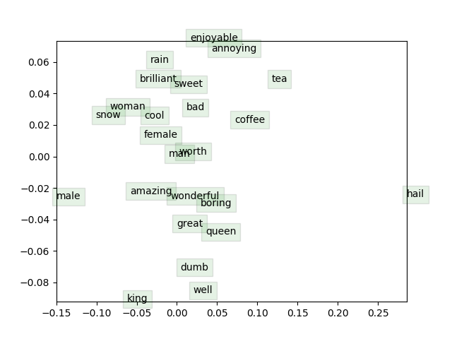
上图是经过训练的词向量的可视化。我们可以注意到一些模式：

近义词被组合在一起，比如 amazing 和 wonderful，woman 和 female。
- 但是 man 和 male 却距离较远
反义词可能因为经常属于同一上下文，它们也会与同义词一起出现，比如 enjoyable 和 annoying。
man:king::woman:queen 以及 queen:king::female:male 形成的两条直线基本平行

Assignment 03¶

1. Machine Learning & Neural Networks¶

(a) Adam Optimizer¶

回忆一下标准随机梯度下降的更新规则 $$ \boldsymbol{\theta} \leftarrow \boldsymbol{\theta}-\alpha \nabla_{\boldsymbol{\theta}}{J_{\mathrm{minibatch}}(\boldsymbol{\theta})} $$ 其中，$\boldsymbol{\theta}$ 是包含模型所有参数的向量，$J$ 是损失函数，$\nabla_{\boldsymbol{\theta}} J_{\mathrm{minibatch}}(\boldsymbol{\theta})$ 是关于minibatch数据上参数的损失函数的梯度，$\alpha$ 是学习率。Adam Optimization使用了一个更复杂的更新规则，并附加了两个步骤。

Question 1.a.i

首先，Adam使用了一个叫做 $momentum$ 动量的技巧来跟踪梯度的移动平均值 $m$

\[ \begin{aligned} \mathbf{m} & \leftarrow \beta_{1} \mathbf{m}+\left(1-\beta_{1}\right) \nabla_{\boldsymbol{\theta}} J_{\text { minibatch }}(\boldsymbol{\theta}) \\ \boldsymbol{\theta} & \leftarrow \boldsymbol{\theta}-\alpha \mathbf{m} \end{aligned} \]

其中，$\beta_1$ 是一个 0 和 1 之间的超参数(通常被设为0.9)。简要说明(不需要用数学方法证明，只需要直观地说明)如何使用m来阻止更新发生大的变化，以及总体上为什么这种小变化可能有助于学习。

Answer 1.a.i :

由于超参数 $\beta _1$ 一般被设为0.9，此时对于移动平均的梯度值 $m$ 而言，主要受到的是之前梯度的移动平均值的影响，而本次计算得到的梯度将会被缩放为原来的 ${1 - \beta_1}$ 倍，即时本次计算得到的梯度很大（梯度爆炸），这一影响也会被减轻，从而阻止更新发生大的变化。
通过减小梯度的变化程度，使得每次的梯度更新更加稳定，从而使模型学习更加稳定，收敛速度更快，并且这也减慢了对于较大梯度值的参数的更新速度，保证其更新的稳定性。

Question 1.a.ii

Adam还通过跟踪梯度平方的移动平均值 $v$ 来使用自适应学习率

\[ \begin{aligned} \mathbf{m} & \leftarrow \beta_{1} \mathbf{m}+\left(1-\beta_{1}\right) \nabla_{\boldsymbol{\theta}} J_{\text { minibatch }}(\boldsymbol{\theta}) \\ \mathbf{v} & \leftarrow \beta_{2} \mathbf{v}+\left(1-\beta_{2}\right)\left(\nabla_{\boldsymbol{\theta}} J_{\text { minibatch }}(\boldsymbol{\theta}) \odot \nabla_{\boldsymbol{\theta}} J_{\text { minibatch }}(\boldsymbol{\theta})\right) \\ \boldsymbol{\theta} & \leftarrow \boldsymbol{\theta}-\alpha \odot \mathbf{m} / \sqrt{\mathbf{v}} \end{aligned} \]

其中，$\odot, /$ 分别表示逐元素的乘法和除法（所以 $z \odot z$ 是逐元素的平方），$\beta_2$ 是一个 0 和 1 之间的超参数(通常被设为0.99)。因为Adam将更新除以 $\sqrt v$ ，那么哪个模型参数会得到更大的更新？为什么这对学习有帮助？

Answer 1.a.ii :

移动平均梯度最小的模型参数将得到较大的更新。
一方面，将梯度较小的参数的更新变大，帮助其走出局部最优点（鞍点）；另一方面，将梯度较大的参数的更新变小，使其更新更加稳定。结合以上两个方面，使学习更加快速的同时也更加稳定。

(b) Dropout¶

Dropout 是一种正则化技术。在训练期间，Dropout 以 $p_{drop}$ 的概率随机设置隐藏层 $h$ 中的神经元为零(每个minibatch中 dropout 不同的神经元),然后将 $h$ 乘以一个常数 $\gamma$ 。我们可以写为

\[ \mathbf{h}_{\mathrm{drop}}=\gamma \mathbf{d} \circ \mathbf{h} \]

其中，$d \in \{0,1\}^{D_h}$ ( $D_h$ 是 $h$ 的大小)是一个掩码向量，其中每个条目都是以 $p_{drop}$ 的概率为 0 ，以 $1 - p_{drop}$ 的概率为 1。$\gamma$ 是使得 $h_{drop}$ 的期望值为 $h$ 的值

\[ \mathbb{E}_{p_{\text{drop}}}\left[\mathbf{h}_{\text{drop}}\right]_{i}=h_{i}, \text{for all } i \in \{1,\dots,D_h\} \]

Question 1.b.i

$\gamma$ 必须等于什么(用 $p_{drop}$ 表示) ？简单证明你的答案。

Answer 1.b.i :

\[ \gamma = \frac{1}{1 - p_{drop}} \\ \]

证明如下：

\[ \sum_i (1 - p_{drop}) h_i = (1 - p_{drop}) E[h] \\ \sum_i[h_{drop}]_i = \gamma\sum_i (1 - p_{drop}) h_i = \gamma (1 - p_{drop}) E[h] = E[h] \]

Question 1.b.ii

为什么我们应该只在训练时使用 dropout 而在评估时不使用？

Answer 1.b.ii :

如果我们在评估期间应用 dropout ，那么评估结果将会具有随机性，并不能体现模型的真实性能，违背了正则化的初衷。通过在评估期间禁用 dropout，从而观察模型的性能与正则化的效果，保证模型的参数得到正确的更新。

2. Neural Transition-Based Dependency Parsing¶

在本节中，您将实现一个基于神经网络的依赖解析器，其目标是在UAS(未标记依存评分)指标上最大化性能。

依存解析器分析句子的语法结构，在 head words 和修饰 head words 的单词之间建立关系。你的实现将是一个基于转换的解析器，它逐步构建一个解析。每一步都维护一个局部解析，表示如下

一个存储正在被处理的单词的栈
一个存储尚未处理的单词的缓存
一个解析器预测的依赖的列表

最初,栈只包含 ROOT ，依赖项列表是空的，而缓存则包含了这个句子的所有单词。在每一个步骤中,解析器将对部分解析使用一个转换,直到它的魂村是空的，并且栈大小为1。可以使用以下转换：

SHIFT：将buffer中的第一个词移出并放到stack上。
LEFT-ARC：将第二个(最近添加的第二)项标记为栈顶元素的依赖，并从堆栈中删除第二项
RIGHT-ARC：将第一个(最近添加的第一)项标记为栈中第二项的依赖，并从堆栈中删除第一项

在每个步骤中，解析器将使用一个神经网络分类器在三个转换中决定。

Question 2.a

求解解析句子 “I parsed this sentence correctly” 所需的转换顺序。这句话的依赖树如下所示。在每一步中，给出 stack 和 buffer 的结构，以及本步骤应用了什么转换，并添加新的依赖(如果有的话)。下面提供了以下三个步骤。

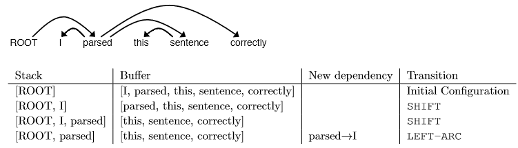
Answer 2.a :

Stack	Buffer	New dependency	Transition
[ROOT]	[I, parsed, this, sentence, correctly]		Initial Conﬁguration
[ROOT, I]	[parsed, this, sentence, correctly]		SHIFT
[ROOT, I, parsed]	[this, sentence, correctly]		SHIFT
[ROOT, parsed]	[this, sentence, correctly]	parsed $\to$ I	LEFT-ARC
[ROOT, parsed, this]	[sentence, correctly]		SHIFT
[ROOT, parsed, this, sentence]	[correctly]		SHIFT
[ROOT, parsed, sentence]	[correctly]	sentence $\to$ this	LEFT-ARC
[ROOT, parsed]	[correctly]	parsed $\to$ sentence	RIGHT-ARC
[ROOT, parsed, correctly]	[]		SHIFT
[ROOT, parsed]	[]	parsed $\to$ correctly	RIGHT-ARC
[ROOT]	[]	ROOT $\to$ parsed	RIGHT-ARC

Question 2.b

一个包含 $n$ 个单词的句子需要多少步(用 $n$ 表示)才能被解析？简要解释为什么。

Answer 2.b :

包含$n$个单词的句子需要 $2 \times n$ 步才能完成解析。因为需要进行 $n$ 步的 $SHIFT$ 操作和共计$n 步的 LEFT-ARC 或 RIGHT-ARC 操作，才能完成解析。（每个单词都需要一次SHIFT和ARC的操作，初始化步骤不计算在内）

Question 2.c

实现解析器将使用的转换机制

Question 2.d

我们的网络将预测哪些转换应该应用于部分解析。我们可以使用它来解析一个句子，通过应用预测出的转换操作，直到解析完成。然而，在对大量数据进行预测时，神经网络的运行速度要高得多(即同时预测了对任何不同部分解析的下一个转换)。我们可以用下面的算法来解析小批次的句子

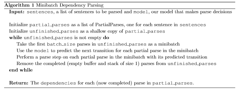
实现minibatch的解析器

我们现在将训练一个神经网络来预测，考虑到栈、缓存和依赖项集合的状态，下一步应该应用哪个转换。首先，模型提取了一个表示当前状态的特征向量。我们将使用原神经依赖解析论文中的特征集合：A Fast and Accurate Dependency Parser using Neural Networks。这个特征向量由标记列表(例如在栈中的最后一个词，缓存中的第一个词，栈中第二到最后一个字的依赖(如果有))组成。它们可以被表示为整数的列表$[w_1,w_2,\dots,w_m]$，m是特征的数量，每个 $0 \leq w_i \lt |V|$ 是词汇表中的一个token的索引($| V |$是词汇量)。首先，我们的网络查找每个单词的嵌入，并将它们连接成一个输入向量：

\[ \mathbf{x}=\left[\mathbf{E}_{w_{1}}, \dots, \mathbf{E}_{w_{m}}\right] \in \mathbb{R}^{d m} \]

其中 $\mathbf{E} \in \mathbb{R}^{|V| \times d}$ 是嵌入矩阵，每一行 $\mathbf{E}_w$ 是一个特定的单词 $w$ 的向量。接着我们可以计算我们的预测：

\[ \mathbf h = \text{ReLU}(\mathbf{xW+b_1}) \\ \mathbf l = \text{ReLU}(\mathbf{hU+b_2}) \\ \mathbf {\hat y} = \text{softmax}(l) \]

其中， $\mathbf{h}$ 指的是隐藏层，$\mathbf{l}$ 是其分数，$\mathbf{\hat y}$ 指的是预测结果， $\text{ReLU(z)}=max(z,0)$ 。我们使用最小化交叉熵损失来训练模型

\[ J(\theta) = CE(\mathbf y,\mathbf{\hat y}) = -\sum^3_{i=1}y_i\log\hat y_i \]

训练集的损失为所有训练样本的 $J(\theta)$ 的平均值。

Question 2.f

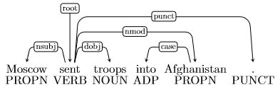
我们想看看依赖关系解析的例子，并了解像我们这样的解析器在什么地方可能是错误的。例如，在这个句子中:

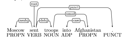
依赖 $\text{into Afghanistan}$ 是错的，因为这个短语应该修饰 $\text{sent}$ (例如 $\text{sent into Afghanistan}$) 而不是 $\text{troops}$ (因为 $\text{ troops into Afghanistan}$ 没有意义)。下面是正确的解析：

一般来说，以下是四种解析错误：

Prepositional Phrase Attachment Error 介词短语连接错误：在上面的例子中，词组 $\text{into Afghanistan}$ 是一个介词短语。介词短语连接错误是指介词短语连接到错误的 head word 上(在本例中，troops 是错误的 head word ，sent 是正确的 head word )。介词短语的更多例子包括with a rock, before midnight和under the carpet。
Verb Phrase Attachment Error 动词短语连接错误：在句子$\text{leave the store alone, I went out to watch the parade}$中，短语 $\text{leave the store alone}$ 是动词短语。动词短语连接错误是指一个动词短语连接到错误的 head word 上(在本例中，正确的头词是 $\text{went}$)。
Modiﬁer Attachment Error 修饰语连接错误：在句子 $\text{I am extremely short}$ 中，副词extremely 是形容词 short 的修饰语。修饰语附加错误是修饰语附加到错误的 head word 上时发生的错误(在本例中，正确的头词是 short)。
Coordination Attachment Error 协调连接错误：在句子 $\text{Would you like brown rice or garlic naan?}$ 中， brown rice 和garlic naan都是连词，or是并列连词。第二个连接词(这里是garlic naan)应该连接到第一个连接词(这里是brown rice)。协调连接错误是当第二个连接词附加到错误的 head word 上时(在本例中，正确的头词是rice)。其他并列连词包括and, but和so。

在这个问题中有四个句子，其中包含从解析器获得的依赖项解析。每个句子都有一个错误，上面四种类型都有一个例子。对于每个句子，请说明错误的类型、不正确的依赖项和正确的依赖项。为了演示:对于上面的例子，您可以这样写：

Error type: Prepositional Phrase Attachment Error
Incorrect dependency: troops $\to$ Afghanistan
Correct dependency: sent $\to$ Afghanistan

注意：依赖项注释有很多细节和约定。如果你想了解更多关于他们的信息，你可以浏览UD网站:http://universaldependencies.org。然而，你不需要知道所有这些细节就能回答这个问题。在每一种情况下，我们都在询问短语的连接，应该足以看出它们是否修饰了正确的head。特别是，你不需要查看依赖项边缘上的标签——只需查看边缘本身就足够了。

Answer 2.f

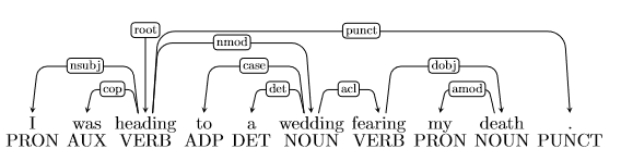
Error type: Verb Phrase Attachment Error
Incorrect dependency: wedding $\to$ fearing
Correct dependency: heading $\to$ fearing

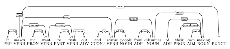
Error type: Coordination Attachment Error
Incorrect dependency: makes $\to$ rescue
Correct dependency: rush $\to$ rescue

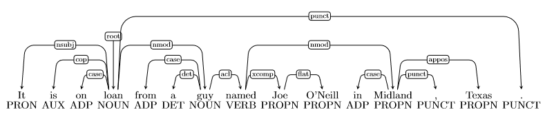
Error type: Prepositional Phrase Attachment Error
Incorrect dependency: named $\to$ Midland
Correct dependency: guy $\to$ Midland

Error type: Modiﬁer Attachment Error
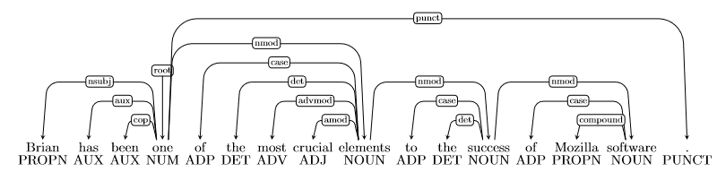
Incorrect dependency: elements $\to$ most
Correct dependency: crucial $\to$ most

Assignment 04¶

1. Neural Machine Translation with RNNs¶

在机器翻译中，我们的目标是将一个句子从源语言(如西班牙语)转换成目标语言(如英语)。在本作业中，我们将注意实现一个序列到序列(Seq2Seq)网络，以建立一个神经机器翻译(NMT)系统。在本节中，我们描述了使用双向LSTM编码器和单向LSTM解码器的NMT系统的训练过程。

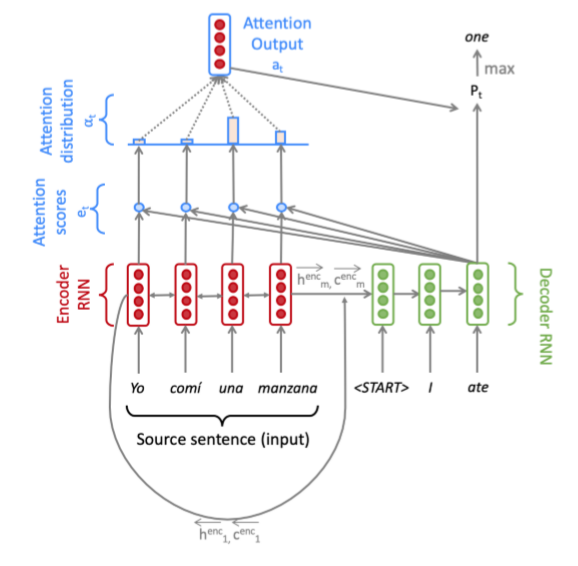
上图是使用乘法注意力的Seq2Seq模型，显示了解码器的第三步。注意，为了可读性，我们不描绘前一个组合输出与解码器输入的连接。

给定源语言中的一个句子，我们从词嵌入矩阵中查找单词嵌入，得到 $\mathbf{x}_{1}, \dots, \mathbf{x}_{m} | \mathbf{x}_{i} \in \mathbb{R}^{e \times 1}$ ，其中 $m$ 为源语句的长度，$e$ 为嵌入大小。我们将这些嵌入提供给双向编码器，为正向($\rightarrow$)和反向($\leftarrow$)LSTMs生成隐藏状态和单元格状态。前向和后向的版本连接起来，以得到隐藏状态 $\mathbf{h}_{i}^{\mathrm{enc}}$ 和单元格状态 $\mathbf{c}_{i}^{\mathrm{enc}}$

\[ \begin{array} \mathbf{h}_{i}^{\mathrm{enc}} = [\overleftarrow {\mathbf{h}_{i}^{\mathrm{enc}}};\overrightarrow {\mathbf{h}_{i}^{\mathrm{enc}}}] \text{ where }\mathbf{h}_{i}^{\mathrm{enc}} \in \mathbb{R}^{2h \times 1} , \overleftarrow {\mathbf{h}_{i}^{\mathrm{enc}}};\overrightarrow {\mathbf{h}_{i}^{\mathrm{enc}}} \in \mathbb{R}^{h \times 1} & 1 \leq i \leq m \\ \mathbf{c}_{i}^{\mathrm{enc}} = [\overleftarrow {\mathbf{c}_{i}^{\mathrm{enc}}};\overrightarrow {\mathbf{c}_{i}^{\mathrm{enc}}}] \text{ where }\mathbf{c}_{i}^{\mathrm{enc}} \in \mathbb{R}^{2h \times 1} , \overleftarrow {\mathbf{c}_{i}^{\mathrm{enc}}};\overrightarrow {\mathbf{c}_{i}^{\mathrm{enc}}} \in \mathbb{R}^{h \times 1} & 1 \leq i \leq m \end{array} \]

然后，我们使用编码器的最终隐藏状态和最终单元状态的线性投影，初始化解码器的第一个隐藏状态 $\mathbf{h}_{0}^{\mathrm{dec}}$ 和单元状态 $\mathbf{c}_{0}^{\mathrm{dec}}$

\[ \begin{array} \mathbf{h}_{0}^{\mathrm{enc}} = [\overleftarrow {\mathbf{h}_{1}^{\mathrm{enc}}};\overrightarrow {\mathbf{h}_{m}^{\mathrm{enc}}}] \text{ where }\mathbf{h}_{0}^{\mathrm{enc}} \in \mathbb{R}^{h \times 1} , \mathbf{W}_{h} \in \mathbb{R}^{h \times 2 h} \\ \mathbf{c}_{0}^{\mathrm{enc}} = [\overleftarrow {\mathbf{c}_{1}^{\mathrm{enc}}};\overrightarrow {\mathbf{c}_{m}^{\mathrm{enc}}}] \text{ where }\mathbf{c}_{0}^{\mathrm{enc}} \in \mathbb{R}^{h \times 1} , \mathbf{W}_{c} \in \mathbb{R}^{h \times 2 h} \end{array} \]

初始化解码器之后，现在必须用目标语言为它提供匹配的句子。在第 $t$ 步，我们查找第 $t$ 个单词的嵌入，$\mathbf{y}_{t} \in \mathbb{R}^{e \times 1}$ 。然后，我们将 $y_t$ 与前一个时间步的 combined-output 组合输出向量 $\mathbf{o}_{t-1} \in \mathbb{R}^{h \times 1}$ 连接起来(我们将在下一页解释这是什么！)，得到 $\overline{\mathbf{y}_{t}} \in \mathbb{R}^{(e+h) \times 1}$ 。注意，对于第一个目标单词(即 start 标记)，$o_0$是一个零向量。然后将 $\overline{\mathbf{y}_{t}}$ 作为输入输入到解码器LSTM中。

\[ \mathbf{h}_{t}^{\mathrm{dec}}, \mathbf{c}_{t}^{\mathrm{dec}}=\text { Decoder }\left(\overline{\mathbf{y}_{t}}, \mathbf{h}_{t-1}^{\mathrm{dec}}\right) \text { where } \mathbf{h}_{t}^{\mathrm{dec}} \in \mathbb{R}^{h \times 1}, \mathbf{c}_{t}^{\mathrm{dec}} \in \mathbb{R}^{h \times 1} \]

然后我们用 $\mathbf{h}_{t}^{\mathrm{dec}}$ 来计算在 $\mathbf{h}_{0}^{\mathrm{enc}}, \ldots, \mathbf{h}_{m}^{\mathrm{enc}}$ 上的乘法注意

\[ \mathbf{e}_{t, i}=\left(\mathbf{h}_{t}^{\mathrm{dec}}\right)^{T} \mathbf{W}_{\mathrm{attProj}} \mathbf{h}_{i}^{\mathrm{enc}} \text { where } \mathbf{e}_{t} \in \mathbb{R}^{m \times 1}, \mathbf{W}_{\mathrm{attProj}} \in \mathbb{R}^{h \times 2 h} \quad \quad 1 \leq i \leq m \\ \alpha_{t}=\operatorname{Softmax}\left(\mathbf{e}_{t}\right) \text { where } \alpha_{t} \in \mathbb{R}^{m \times 1} \\ \mathbf{a}_{t}=\sum_{i}^{m} \alpha_{t, i} \mathbf{h}_{i}^{\mathrm{enc}} \text { where } \mathbf{a}_{t} \in \mathbb{R}^{2 h \times 1} \]

现在，我们将注意力输出 $\alpha_t$ 与解码器隐藏状态 $\mathbf{h}_{t}^{\mathrm{dec}}$ 连接起来，并将其通过线性层 Tanh 和 Dropout 来获得组合输出向量 $o_t$ 。

\[ \begin{aligned} \mathbf{u}_{t} &=\left[\mathbf{a}_{t}; \mathbf{h}_{t}^{\mathrm{dec}}\right] \text { where } \mathbf{u}_{t} \in \mathbb{R}^{3 h \times 1} \\ \mathbf{v}_{t} &=\mathbf{W}_{u} \mathbf{u}_{t} \text { where } \mathbf{v}_{t} \in \mathbb{R}^{h \times 1}, \mathbf{W}_{u} \in \mathbb{R}^{h \times 3 h} \\ \mathbf{o}_{t} &=\operatorname{Dropout}\left(\operatorname{Tanh}\left(\mathbf{v}_{t}\right)\right) \text { where } \mathbf{o}_{t} \in \mathbb{R}^{h \times 1} \end{aligned} \]

然后，在第 $t$ 个时间步长时，得到目标词的概率分布 $\mathbf{P}_{t}$

\[ \mathbf{P}_{t}=\operatorname{Softmax}\left(\mathbf{W}_{\mathrm{vocab}} \mathbf{o}_{t}\right) \text { where } \mathbf{P}_{t} \in \mathbb{R}^{V_{t} \times 1}, \mathbf{W}_{\mathrm{vocab}} \in \mathbb{R}^{V_{t} \times h} \]

这里， $V_t$ 是目标词汇表的大小。最后，为了训练网络，我们计算了 $\mathbf{P}_{t} ,\mathbf{g}_{t}$ 之间的 softmax 交叉熵损失，$\mathbf{g}_{t}$ 是时间步 $t$ 的目标词的 one-hot 向量

\[ J_{t}(\theta)=C E\left(\mathbf{P}_{t}, \mathbf{g}_{t}\right) \]

在这里，$\theta$ 代表所有的模型参数，$J_t(\theta)$是解码器第 $t$ 步的损失。现在我们已经描述了该模型，让我们尝试将其实现为西班牙语到英语的翻译！

Pytorch Bidirectional RNNs Note

Pytorch 中的 RNNs，返回的 out 的 shape 为 $\text{(seq_len, batch, num_directions * hidden_size)}$

转换为 $\text{(seq_len, batch, num_directions, hidden_size)}$ 后，num_directions 中的顺序是先 forward 再 backward，并且 forward 和 backward 的 hidden state 的顺序是相反的，即 $out[0][0][0]$ 是 forward 的第一个时间步的结果，而 $out[0][0][1]$ 是 backward 的最后一个时间步的结果。此外，out 只包含最后一层的结果

但对于 h_n ( c_n 同理) 而言，shape 为 $\text{(num_layers * num_directions, batch, hidden_size)}$ ，保存的是 forward 和 backward 的最后一个时间步的结果。

转换为 $\text{(num_layers, num_directions, batch, hidden_size)}$ 后，第一维的 num_layers 和真实的 layer 层数一一对应，即 $h_n[1][0][0]$ 与 $out[-1][0][0]$ 相等， $h_n[1][1][0]$ 与 $out[0][0][1]$ 。

Question 1.g

首先解释(大约三句话) masks 对整个注意力计算有什么影响。然后(用一两句话)解释为什么有必要这样使用 masks 。

Answer 1.g

使用 masks 将句子中的 pad token 的分数赋值为 $-inf$ ，从而使得 softmax 作用后获得的 attention 分布中，pad token 的 attention 概率值近似为 0
attention score / distributions 计算的是 decoder 中某一时间步上的 target word 对 encoder 中的所有 source word 的注意力概率，而 pad token 只是用于 mini-batch ，并没有任何语言意义，target word 无须为其分散注意力，所以需要使用 masks 过滤掉 pad token

Question 1.j

在课堂上，我们学习了点积注意、乘法注意和加法注意。请就其他两种注意机制中的任何一种，提供每种注意机制可能的优点和缺点

点积注意 $\mathbf{e}_{t, i}=\mathbf{s}_{t}^{T} \mathbf{h}_{i}$
乘法注意 $\mathbf{e}_{t, i}=\mathbf{s}_{t}^{T} \mathbf{W h}_{i}$
加法注意 $\mathbf{e}_{t, i}=\mathbf{v}^{T}(\mathbf{W}_{1} \mathbf{h}_{i}+\mathbf{W}_{2} \mathrm{s}_{t} )$

Answer 1.j

	优点	缺点
点积注意力	不需要额外的线性映射层	$s_t, h_t$ 必须有同样的纬度
乘法注意力	$s_t, h_t$ 不需要有同样的纬度并且因为可以使用高效率的矩阵乘法，比加法注意力要更快更省内存	增加了训练参数
加法注意力	高维时的表现更好	训练参数更多（两个参数矩阵以及注意力的纬度）

2. Analyzing NMT Systems¶

Question 2.a

这里，我们展示了在NMT模型的输出中发现的一系列错误(与您刚刚训练的模型相同)。对于西班牙语源句的每个示例，标准英文翻译，以及NMT(即，“模型”)，请你：

识别NMT翻译中的错误
提供模型可能出错的原因(由于特定的语言构造或特定的模型限制)
描述一种可能的方法，我们可以改变NMT系统，以修复观察到的错误

下面是您应该按照上面描述的那样分析的翻译。请注意，标记了下划线的单词是词汇表外的单词

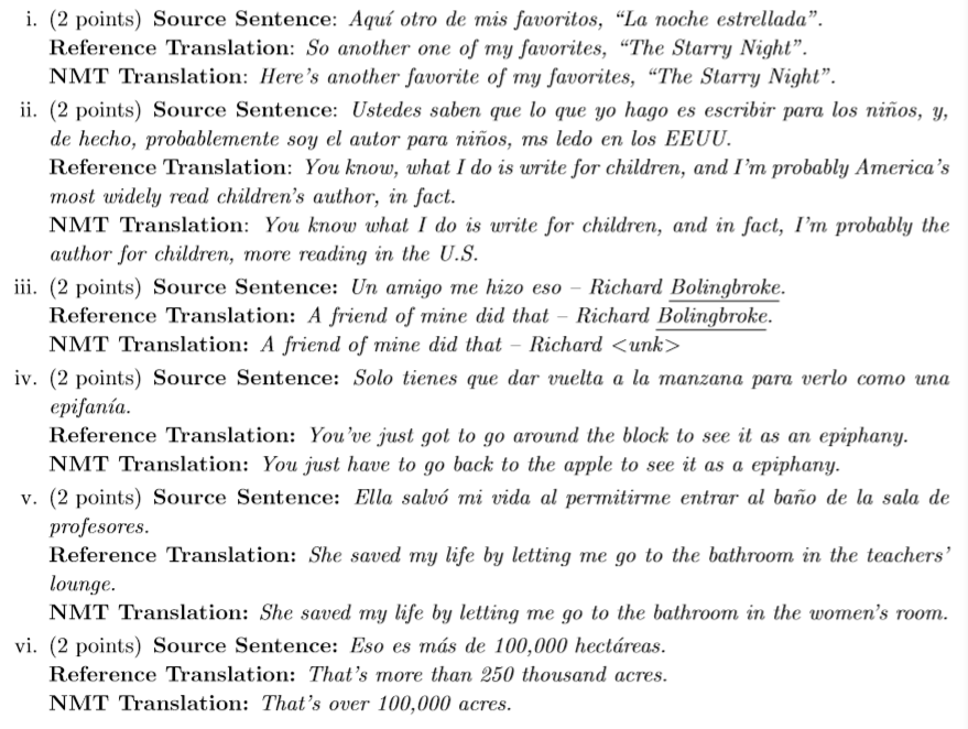
Answer 2.a

Error: “ favorite of my favorites”
Reason: 特定的语言构造，低资源语言对
Possible fix: 尝试在这类语言对上添加更多的训练数据

Error: “ more reading in the U.S.“ 语义错误
Reason: 特定的语言构造，模型对语义的理解不足，需要增大模型的容量以增强理解能力
Possible fix: 增大Hidden_size

Error: ”Richard \<unk>“
Reason: 模型限制，Bolingbroke 是词表外的单词
Possible fix: 对此类姓名中出现的词加以处理，比如直接添加到词表中

Error: ”go back to the apple “
Reason: 模型限制，”manzana“ 有丰富的含义，包括 apple 苹果和 block 街区。“block”在西班牙语中的表达方式比 “apple” 在西班牙语中的表达方式更多。然而，在训练集中，“manzana”更多地表示“apple”，而不是“block”。
Possible fix: 在训练集中添加更多的关于 ”manzana“ 表示 “block” 的数据，保持多重含义的训练不失衡

Error: “go to the bathroom in the women’s room“
Reason: 模型限制，由于在数据集中，女性比专业人员(教师)的出现频率要更高，所以导致翻译具有来自训练数据的偏见 bias
Possible fix: 添加更多 profesore 的训练样本

Error: ”100,000 acres.“
Reason: 模型限制，常识错误，hectáreas 表示公顷，acres 表示英亩（acre的复数）。模型并未理解两个单位制之间的转换关系，由于 acres 在训练集中的出现频率更高，直接采用 acres 并且使用 hectáreas 附近的数字直接修饰 acres
Possible fix: 添加关于 hectáreas 的训练数据

Question 2.b

现在是时候探索您所训练的模型的输出了！问题 1-i 中生成的模型的测试集翻译应该位于output /test_output.txt中。请找出你的模型产生的两个错误示例。你发现的两个例子应该是不同的错误类型，并且与前一个问题中提供的例子不同。对于每个例子，你应该：

写下西班牙语原文句子。源语句在 en_es_data/test.es 中
写下参考译文，参考译文在en_es_data/test.en中
写下NMT模型的英文翻译，模型翻译的句子位于output /test_output .txt中
识别NMT翻译中的错误
提供模型可能出错的原因(由于特定的语言构造或特定的模型限制)
描述一种可能的方法，我们可以改变NMT系统，以修复观察到的错误

Answer 2.b

Source Sentence: El 5 de noviembre de 1990
Reference Translation: On November 5^th, 1990
NMT Translation: On five of November 1990
Error: five
Reason: 模型限制，模型没有数据集中充分学习到日期格式的转换
Possible Fix: 增加更多关于西班牙语与英语之间的日期格式转换的数据样本

Source Sentence: Y mis amigos hondureos me pidieron que dijera: "Gracias TED".
Reference Translation: And my friends from Honduras asked me to say thank you, TED.
NMT Translation: My friends were asked to say, "Thank you."
Error : 说话的对象错误，说话的人是我而不是我的朋友
Reason: 句法结构有误并且有缺译现象
Possible Fix: 尝试为模型的添加更有效的对齐方式，如优化注意力模型

Question 2.c

BLEU评分是NMT系统中最常用的自动评价指标。它通常在整个测试集中计算，但这里我们将考虑为单个示例定义的BLEU。假设我们有一个源句 $s$ ，一组 $k$ 个参考译文 $\mathbf{r}_{1}, \dots, \mathbf{r}_{k}$ 和一个候选翻译 $\boldsymbol{c}$ 。为了计算 $\boldsymbol{c}$ 的BLEU分数，我们首先为 $\boldsymbol{c}$ 计算修改后的 n-gram 精度 $p_{n}$ ，对于 $n = 1,2,3,4$ :

\[ p_{n}=\frac{\sum_{\text{ngram} \in c} \min \left(\max _{i=1, \ldots, k} \operatorname{Count}_{r_{i}}(\text { ngram }), \text {Count}_c \text{(ngram)}\right)}{\sum_{\text{ngram} \in c} \text {Count}_c \text{(ngram)}} \]

这里，对于出现在候选翻译 $\boldsymbol{c}$ 中的每个 n-gram ，我们计算它在任何一个参考译文中出现的最大次数，并以它出现在 $\boldsymbol{c}$ 中的次数为上限(这是分子)，再除以 $\boldsymbol{c}$ 的 n-gram (分母)

接下来，我们计算简洁代价 $\text{brevity penalty BP}$ 。令 $c$ 作为 $\boldsymbol{c}$ 的长度，让 $r^*$ 作为最接近 $\boldsymbol{c}$ 的参考翻译的长度(在两个相等接近的参考翻译长度的情况下，选择较短的参考翻译的长度作为 $r^*$ )

\[ B P=\left\{\begin{array}{ll}{1} & {\text { if } c \geq r^{*}} \\ {\exp \left(1-\frac{r^{*}}{c}\right)} & {\text { otherwise }}\end{array}\right. \]

最后，候选翻译 $\boldsymbol{c}$ 关于 $\mathbf{r}_{1}, \dots, \mathbf{r}_{k}$ 的BLEU分数为：

\[ B L E U=B P \times \exp \left(\sum_{n=1}^{4} \lambda_{n} \log p_{n}\right) \]

其中，$\lambda_{1}, \lambda_{2}, \lambda_{3}, \lambda_{4}$ 是总和为1的权重

Question 2.c.i

请考虑这个例子：

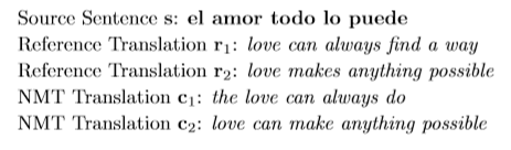
分别计算 $c_1, c_2$ 的BLEU分数。令 $\lambda_{i}=0.5 \text { for } i \in\{1,2\}, \lambda_{i}=0 \text { for } i \in\{3,4\}$ 。当计算BLEU分数时，显示你的计算过程(展示 $p_1, p_2, c, r^{*}, BP$ 的计算值)。

根据BLEU评分，这两种NMT翻译中哪一种被认为是更好的翻译?你同意这是更好的翻译吗？

Answer 2.c.i

$c_1$

\[ \begin{array}{l} {p_1} &= \frac{0+1+1+1+0}{5} = 0.6 \\ {p_2} &= \frac{0+1+1+0}{4} = 0.5 \\ c &= 5 \\ r^* &= 4 \\ BP &= 1 \\ BLEU_{{c_1}} &= 1 * \exp(0.5 * \log(0.6) + 0.5 * \log(0.5)) = 0.5477 \end{array} \]

$c_2$

\[ \begin{array}{l} {p_1} &= \frac{1+1+0+1+1}{5} = 0.8 \\ {p_2} &= \frac{1+0+0+1}{4} = 0.5 \\ c &= 5 \\ r^* &= 4 \\ BP &= 1 \\ BLEU_{{c_1}} &= 1 * \exp(0.5 * \log(0.8) + 0.5 * \log(0.5)) = 0.632 \end{array} \]

根据 BLEU 分数，$c_2$ 是得分更高的翻译，但我认为 $c_1$ 的翻译更加好

Question 2.c.ii

我们的硬盘坏了，我们失去了参考翻译 $r_2$ 。请重新计算 $c_1$ 和 $c_2$ 的BLEU分数，这次只针对 $r_1$ 。两个NMT分一中，哪一个现在获得了更高的BLEU分数？你同意这是更好的翻译吗？

Answer 2.c.ii

$c_1$

\[ \begin{array}{l} {p_1} &= \frac{0+1+1+1+0}{5} = 0.6 \\ {p_2} &= \frac{0+1+1+0}{4} = 0.5 \\ c &= 5 \\ r^* &= 6 \\ BP &= \exp(1 - \frac{6}{5}) = 0.8187 \\ BLEU_{{c_1}} &= 0.8187 * \exp(0.5 * \log(0.6) + 0.5 * \log(0.5)) = 0.4484 \end{array} \]

$c_2$

\[ \begin{array}{l} {p_1} &= \frac{1+1+0+0+0}{5} = 0.4 \\ {p_2} &= \frac{1+0+0+0}{4} = 0.25 \\ c &= 5 \\ r^* &= 6 \\ BP &= \exp(1 - \frac{6}{5}) = 0.8187 \\ BLEU_{{c_1}} &= 0.8187 * \exp(0.5 * \log(0.4) + 0.5 * \log(0.25)) = 0.2589 \end{array} \]

根据 BLEU 分数，$c_1$ 是得分更高的翻译，并且我认为这是对的

Question 2.c.iii

由于数据可用性，NMT系统通常只根据一个参考翻译进行评估。请解释(用几句话)为什么这可能有问题？

Answer 2.c.iii

如果我们使用单一参考翻译，它增加了好翻译由于与单一参考翻译有较低的 n-gram overlap ，而获得较差的BUEU分数的可能性。例如上例中，如果删去的参考翻译是 $r_1$ ，那么将使得 $c_1$ 的BLEU分数变低。

如果我们增加更多的参考翻译，就会增加一个好翻译中 n-gram overlap 的几率，这样我们就有可能使好翻译获得相对较高的BLEU分数。

Question 2.c.iv

列举了BLEU作为机器翻译的评价指标，相对于人工评价的两个优点和两个缺点。

Answer 2.c.iv

优点

自动评价，比人工评价更快，方便，快速
BLEU的使用普及率较高，方便模型之间的效果对比

缺点

结果并不稳定，由于核心思想是 n-gram overlap，所以如果参考翻译不够丰富，会导致出现较好翻译获得较差BLEU分数的情况
不考虑语义与句法
不考虑词法，例如上例中的make和makes
未对同义词或相似表达进行优化

	优点	缺点
点积注意力	不需要额外的线性映射层	\(s_t, h_t\) 必须有同样的纬度
乘法注意力	\(s_t, h_t\) 不需要有同样的纬度并且因为可以使用高效率的矩阵乘法，比加法注意力要更快更省内存	增加了训练参数
加法注意力	高维时的表现更好	训练参数更多（两个参数矩阵以及注意力的纬度）